


Helios | You are my Sunshine
Morelia, Michoacán
Team Updates
See our website regarding our progress on this challenge:
http://www.ifm.umich.mx/~jedwards/nasa.html
You can download our report on our work at that site and find our open source code for the data from HI-SEAS!
T
Thomai TsiftsiSee our website regarding our progress on this challenge:
http://www.ifm.umich.mx/~jedwards/nasa.html
You can download our report on our work at that site!
J
James Edwards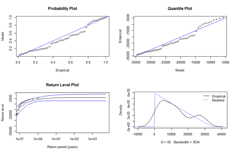
Paretofinal.png
J
James Edwards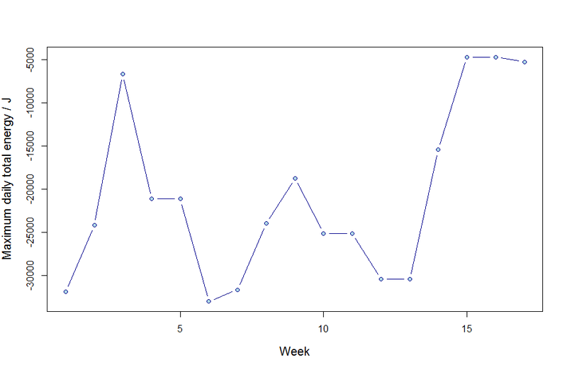
weeklyenergy.png
J
James Edwards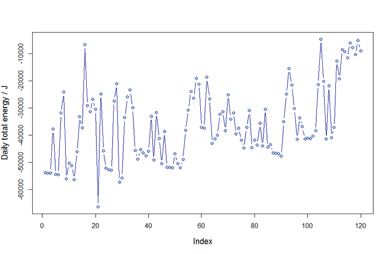
Dailyenergy.png
J
James Edwards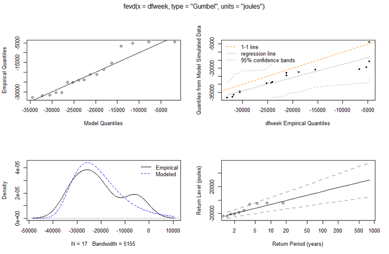
GEVGumbel.png
J
James Edwards| \documentclass[11pt,a4paper]{article} | |
| \usepackage[utf8]{inputenc} | |
| \usepackage{amsmath} | |
| \usepackage{amsfonts} | |
| \usepackage{amssymb} | |
| \usepackage{graphicx} | |
| \usepackage[lmargin=2.4cm, rmargin=2.4cm, tmargin=2.6cm, bmargin=2.4cm]{geometry} | |
| \usepackage{subfig} | |
| \title{Nasa SpaceApps challenge} | |
| \author{Dr. Thomai Tsiftsi, Dr James P. Edwards, Dr Gourouni Ph.D.,\\ Det Sup. Leodaris Edwards, H Mouma Edwards} | |
| \begin{document} | |
| \maketitle | |
| In this challenge we examine the Hi-SEAS solar radiation data and employ extreme value analysis to describe the probabilities of extreme values. In particular, we focus on asymptotic analysis of the distributions of particularly low total daily radiation output of the solar panels. The motivation of this analysis is to facilitate the Hi-SEAS crew planning for the possibility of extreme drops in solar panel output (due to natural variation in weather, radiation output and other factors), ensuring that sufficient power reserves are maintained to cope with extreme lows. | |
| The analyse our data we began by estimating the total daily output by approximating the total energy generated by the cells as a discretisation of the time integral of the flux power, | |
| \begin{equation} | |
| x_{i} = \sum_{k = 1}^{N} \, 72 \times p_{ik} \times\frac{t_{i,k+1} - t_{i,k}}{3600} \times\mathcal{E} | |
| \end{equation} | |
| where $\mathcal{E} \approx0.1$ is the estimated efficiency of the solar cells which have area $72m^{2}$. The sum is over the given data points, $p_{ik}$, representing the solar radiation flux on day $i$ at time $t_{i,k}$. In anticipation of extreme value analysis, we also blocked these data into weekly observations, $\{x_{1}, \ldots, x_{n = 7}\}$. These data are displayed below in figure (\ref{figdat}) | |
| \begin{figure} | |
| \centering | |
| \subfloat[][The estimated total daily energy output by Hi-SEAS polar panels for 120 days.] | |
| { | |
| \includegraphics[width=0.45\textwidth]{DailyEnergy.png} | |
| } | |
| \subfloat[][The maximum daily energy output in each week during the same period.] | |
| { | |
| \includegraphics[width=0.45\textwidth]{weeklyEnergy.png} | |
| } | |
| \caption{Daily maxima and the weekly maxima energy output.} | |
| \label{figdat} | |
| \end{figure} | |
| \subsection*{Generalised extreme value theory} | |
| Let $M_{i} = \textrm{max}\{ x_{1}, \ldots, x_{n}\}$. Then extreme value analysis states that the asymptotic distribution of $M_{n}$, if it exists, must take the form (GEV) | |
| \begin{equation} | |
| \mathcal{P}(M_{i} \leq z) \simeq G(z | \mu, \sigma, \xi) \equiv\exp{\left[ - \left(1 + \xi\left(\frac{z-\mu}{\sigma}\right)^{-\frac{1}{\xi}} \right) \right]}, | |
| \end{equation} | |
| for parameters $\mu$, location, $\sigma$, scale, and shape, $\xi$. These parameters can be fitted to our data, following which $G(z)$ provides an asymptotic estimate of the tails of the distribution of the maxima of a set of data. Here we are interested in \textit{minima} so we must take our daily accumulated energies and \textit{negate} them so that minima become (negative) maxima. | |
| Fitting our data to the model initially provided \textit{maximum likelihood\footnote{The likelihood for the data given the model is\begin{equation}-N\log(\sigma) - (1 + \frac{1}{\xi})\sum_{i=1}^{N}\left[\log{\left(1 + \xi\left(\frac{z_{i} - \mu}{\sigma}\right)\right)} - \left(1 + \xi\left(\frac{z_{i} - \mu}{\sigma}\right)\right)^{-\frac{1}{\xi}} \right]\end{equation} where $z_{i}$ are the empirical maxima. The case $\xi = 0$ is treated as the limiting form of $G(z | \mu, \sigma, \xi\rightarrow0)$. The likelihood is maximised with respect to the parameters $\mu$, $\sigma$, $\xi$.}} estimates of the parameters | |
| \begin{center} | |
| \begin{tabular}{|c|c|c|c|} | |
| \hline | |
| & $\mu$ & $\sigma$ & $\xi$\\ | |
| \hline | |
| Estimate & $-2.6\times10^{4}$ & $48.3\times10^{3}$ & $3.9\times10^{-2}$\\ | |
| \hline | |
| Std Err& $2.3\times10^{3}$ & $2.8\times10^{3}$ & $4.6\times10^{-1}$\\ | |
| \hline | |
| \end{tabular} | |
| \end{center} | |
| However, one notes that the shape parameter has large standard errors making its estimate compatible with $0$. For this reason we re-fit the data to the subset of models with vanishing shape parameter (Gumbel distribution); the likelihood ratio test provided a $p$-value of $0.89$ on a null hypothesis of $\xi = 0$, giving sufficient evidence to accept it. This lead to a refined model with fewer parameters, whose estimates are | |
| \begin{center} | |
| \begin{tabular}{|c|c|c|} | |
| \hline | |
| & $\mu$ & $\sigma$\\ | |
| \hline | |
| Estimate & $-2.6\times10^{4}$ & $8.3\times10^{3}$\\ | |
| \hline | |
| Std Err& $2.1\times10^{3}$ & $1.8\times10^{3}$\\ | |
| \hline | |
| \end{tabular} | |
| \end{center} | |
| which are used as estimates for prediction of extreme daily energy outputs per week. | |
| The plot in figure \ref{figGum} gives diagnostic and predictive results for the data. The probability distribution function at at $z$ gives the probability that $M_{n}$ will be within an infinitesimal interval, $dz$ of $z$. Of particular interest for Hi-SEAS is the \textbf{return level} plot (and associated confidence intervals). The $m^{th}$ return level is the value of the daily energy so \textit{low} that it is \textit{exceeded} once every $m$ observations, here translated into numbers of years. We summary various results of special interest in the table below: | |
| \begin{center} | |
| \begin{tabular}{|c|c|c|c|} | |
| \hline | |
| & Estimate & Lower confidence interval & Upper confidence interval \\ | |
| \hline | |
| 2 years & 17.9 kJ & 23.9kJ & 22.7kJ \\ | |
| \hline | |
| 3 years & 18.1kJ & 12.2kJ & 24.0kJ \\ | |
| \hline | |
| 4 years & 15.2kJ & 8.4kJ & 22.0kJ \\ | |
| \hline | |
| 5 years & 13.1kJ& 5.6kJ & 20.6kJ \\ | |
| \hline | |
| \end{tabular} | |
| \end{center} | |
| As an example, once every 4 years, we expect to see a total daily flux of $8.4$kJ or less. | |
| \begin{figure} | |
| \centering | |
| \includegraphics[width=0.75\textwidth]{GEVGumbel.png} | |
| \caption{Diagnostics for the GEV fitting procedure.} | |
| \label{figGum} | |
| \end{figure} | |
| \subsection*{Threshold excesses} | |
| Examining only the minima of the daily temperatures each week does not take full advantage of the dataset. For this reason, an alternative asymptotic analysis to extreme events is to determine the limiting distribution of $\mathcal{P}(X < u |X < u_{0})$ where $u_{0}$ is a sufficiently large parameter and $X$ represents the daily energy output. If the asymptotic limit of this distribution exists it takes the form of a generalised Pareto distribution, | |
| \begin{equation} | |
| H(y \equiv x - u) = 1 - \left(1 + \frac{\xi y}{\tilde{\sigma}}\right)^{-\frac{1}{\xi}}, | |
| \end{equation} | |
| where $\tilde{\sigma} = \sigma + \xi(u - \mu)$ and we fit the parameters $\xi$ and $\tilde{\sigma}$ from the data. By empirically estimating $\zeta_{u_{0}} \equiv\mathcal{P}(X < u_{0})$ one can assign probabilities to | |
| \begin{equation} | |
| \mathcal{P}(X > u > u_{0}) \approx\zeta_{u_{0}}H(x - u). | |
| \end{equation} | |
| The threshold, $u_{0}$ must be sufficiently large that $\tilde{\sigma}$ is constant with respect to $u$. We found in our data that $u_{0} \approx35,000$ satisfies this condition within the $95\%$ confidence interval. Our maximum likelihood analysis\footnote{If $K$ observations are above the threshold by amounts $y_{i} = x_{i} - u_{0}$ then the likelihood is easily found to be \begin{equation}-K\log(\sigma) - (1 + \frac{1}{\xi})\sum_{i = 1}^{K}\log{\left(1 + \frac{\xi y_{i}}{\tilde{\sigma}}\right)}\end{equation} with the $\xi = 0$ limit following from a limiting procedure.} yielded the following parameters | |
| \begin{center} | |
| \begin{tabular}{|c|c|c|} | |
| \hline | |
| & $\mu$ & $\sigma$\\ | |
| \hline | |
| Estimate & $1.7\times10^{4}$ & $4.8\times10^{-1}$\\ | |
| \hline | |
| Std Err& $3.2\times10^{3}$ & $1.7\times10^{-1}$\\ | |
| \hline | |
| \end{tabular} | |
| \end{center} | |
| It is an unfortunate artifact of the relatively small number of days in the dataset (120 days, approximately 17 weeks) and the rudimentary estimate of the total daily energy output that these parameters are not compatible with those of the GEV above. | |
| Diagnostic plots provide the post-hoc justification of our analysis -- figure (\ref{figP}). In particular, the probability distribution function provides estimates of finding $X - u$ within an infinitesimal region, $dy$ of the value $y$. Return level plots give the value of the daily output that occurs once every $m$ observations, here given in years. | |
| \begin{figure} | |
| \centering | |
| \includegraphics[width=0.75 \textwidth]{Paretoextremes.png} | |
| \end{figure} | |
| \end{document} |
J
James Edwards| # set directory | |
| setwd("C:/Users/Thomai/Desktop/NASA") | |
| ### load the data for pressure, humidity, solar radiation, temperature, wind direction, wind speed | |
| barpres<- read.table("barometric pressure.csv", header=FALSE,sep=",") | |
| hum= read.table("humidity.csv", header=FALSE,sep=",") | |
| solra= read.table("solar radiation.csv", header=FALSE,sep=",") | |
| temp= read.table("temperature.csv", header=FALSE,sep=",") | |
| winddir= read.table("wind direction in degrees.csv", header=FALSE,sep=",") | |
| windspeed= read.table("wind speed.csv", header=FALSE,sep=",") | |
| sunrise= read.table("sunrise.csv", header=FALSE,sep=",") | |
| sunset= read.table("sunset.csv", header=FALSE,sep=",") | |
| # create a data frame of the data with common unixtime, date, local time | |
| dfmain=data.frame(barpres[,1:5], hum[,5],solra[,5], temp[,5],winddir[,5],windspeed[,5]) | |
| dfmain=dfmain[,2:10] | |
| dfsuntimes=data.frame(sunrise[,2:5],sunset[,5]) | |
| # create the column names for our data | |
| colnames(dfmain) = c("unixtime", "date", "localtime", "bar. pressure", "humidity","sol. radiation","temperature","wind direction", "wind speed") | |
| colnames(dfsuntimes) = c("unixtime", "date", "localtime","sunrise","sunset") | |
| ### find the number of observations per day | |
| # u finds the unique dates in the column called date | |
| u= unique(dfmain[,2]) | |
| #dim(dfmain[dfmain$date == "2016-09-29",])[1] | |
| dfdays=c(0,0,0,0) | |
| # calculating the daily energy outcome by finding unique days | |
| for (dtinu) | |
| { | |
| print(dt) | |
| x=dfmain[dfmain$date==dt,] | |
| avrt=0 | |
| tot=c(0,0,0) | |
| for( iin1:(dim(x)[1]-1)) | |
| { | |
| delt=72*x[i,6] * (x[i+1,1] -x[i,1])/(3600) | |
| tot[1] = (tot[1] +delt*0.1) | |
| tot[2] = (tot[2] +delt*0.08) | |
| tot[3] = (tot[3] +delt*0.12) | |
| } | |
| dfdays=(rbind(dfdays, c(dt,tot[1],tot[2],tot[3]))) | |
| } | |
| # extract the first row of zeros | |
| dfdays=dfdays[-1,] | |
| #plot the daily energy outcome | |
| plot(dfdays[,2],type="b", xlab="Index", ylab="Daily total energy / J", cex.lab=1.25, col="darkblue",bg="lightblue", pch=21) | |
| #### do EVT in the minima (which we have negated to have as maxima) | |
| library(ismev) | |
| library(extRemes) | |
| # turn the energy values into numeric | |
| dat= as.numeric(dfdays[,2]) | |
| dfweek= rep(0, floor(length(dat)/7)) | |
| #block the data into weeks and extract the weekly maxima | |
| for(jin1:floor(length(dat)/7)) | |
| { | |
| wk=dat[(7*(j-1)):(7*j)] | |
| dfweek[j] = max(wk); | |
| } | |
| # plot maxima per week | |
| plot(dfweek,type="b", xlab="Week", ylab="Maximum daily total energy / J", cex.lab=1.25, col="darkblue",bg="lightblue", pch=21) | |
| # perform the EVT analysis using package ismev | |
| A= gev.fit(dfweek) | |
| #diagnostic plots | |
| gev.diag(A) | |
| # perform EVT analysis using package extremes | |
| fitweeks= fevd(dfweek,units="joules") | |
| # diagnostic plots | |
| plot(fitweeks) | |
| # Plots of the likelihood and its gradient for each parameter (holding the other parameters fixed | |
| # ath their MLE estimates) | |
| plot(fitweeks,"trace") | |
| # parameter estimates and their CIs | |
| ci(fitweeks,type="parameter") | |
| ## the two-year return level corresponds to the median of the GEV | |
| return.level(fitweeks) | |
| # return levels and their CIs | |
| return.level(fitweeks,do.ci=TRUE) | |
| # return levels and their CIs for a given period of 2,3,4,5 years | |
| ci(fitweeks,return.period= c(2,3,4,5)) | |
| #There are two ways we can test about the Gumbel hypothesis. The easiest is to use | |
| # the following line of code which gives CI for each parameter estimate (default used below gives the 95% CI) which | |
| #reveals that we reject the null hypothesis of a light tailed df in favour of the upper bounded type. | |
| # our previous shape estimate is too close to zero so fit Gumbel and then compare models. | |
| fitweeksgumb= fevd(dfweek,type="Gumbel", units="joules") | |
| #summary of model | |
| fitweeksgumb | |
| #diagnostic plots | |
| plot(fitweeksgumb) | |
| # trace from model | |
| plot(fitweeksgumb,"trace") | |
| #return levels for Gumbel model | |
| return.level(fitweeksgumb) | |
| #return levels for Gumbel model and their CIs | |
| return.level(fitweeksgumb,do.ci=TRUE) | |
| #parameter estimates for Gumbel model and their CIs | |
| ci(fitweeksgumb,type="parameter") | |
| #return levels for Gumbel model for given periods of time | |
| ci(fitweeksgumb,return.period= c(2,3,4,5)) | |
| ## use likel. test to find which of the two models is favoured.Since p>a then do not reject the null (Gumbel) | |
| # The results of the test provide do not support for rejecting the null hypothesis | |
| # of the Gumbel. | |
| lr.test(fitweeksgumb, fitweeks) | |
| # calculate the probabilities of having energies less | |
| pextRemes(fitweeksgumb, q= c(-10000,0), lower.tail=FALSE) | |
| ############################## TRYING WITH EXCESSES | |
| # turn days into numerical | |
| days= as.numeric(dfdays[,2]) | |
| #choose threshold for our excesses | |
| mrl.plot(days) | |
| # confirm the above chosen threshold | |
| threshrange.plot(days, r= c(-60000,-20000), nint=50) | |
| # fit a generalised Pareto distribution on the excesses | |
| fitD= fevd(days, threshold=-35000, type="GP", time.units="days") | |
| plot(fitD) | |
| ci(fitD,type="parameter") | |
| ci(fitD,return.period= c(2,3,4,5)) | |
| fitexp= fevd(days,threshold=-35000, type="Exponential", time.units="days", verbose=TRUE) | |
| #fit it with package ismev | |
| test= gpd.fit(days,threshold=-35000, npy=120, show=TRUE) | |
| gpd.diag(test) | |
T
Thomai Tsiftsi| Fitting our data to the model initially provided \textit{maximum likelihood\footnote{The likelihood for the data given the model is | |
| \begin{equation} | |
| -m\log(\sigma) - (1 + \frac{1}{\xi})\sum_{i}\left[\log{\left(1 + \xi\left(\frac{z_{i} - \mu}{\sigma}\right)\right)} - \left(1 + \xi\left(\frac{z_{i} - \mu}{\sigma}\right)\right)^{-\frac{1}{\xi}} \right]\end{equation} | |
| where $z_{i}$ are the empirical maxima. | |
| The case $\xi = 0$ is treated as the limiting form of $G(z | \mu, \sigma, \xi\rightarrow0)$. The likelihood is maximised with respect to the parameters $\mu$, $\sigma$, $\xi$.}} | |
| estimates of the parameters.... |
J
James Edwards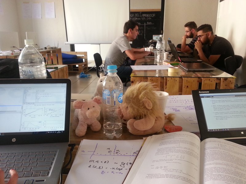
With some help from our friends
J
James Edwards
Hit it with maths...hard
J
James Edwards| dfweek = rep(0, floor(length(dat)/7)) | |
| dat = as.numeric(dfdays[,2]) | |
| for(j in1:floor(length(dat)/7)) | |
| { | |
| wk = dat[(7*(j-1)):(7*j)] | |
| dfweek[j] = max(wk); | |
| } |
J
James Edwards
Analysis diagnostics
J
James Edwards
Hard at work
J
James Edwards
SpaceApps is a NASA incubator innovation program.